Markov Chains — Regime Detection Framework

I am going to break down how hedge funds use Markov Chains to find high probability winning trades consistently & share the exact framework you can start building today. Let’s get straight to it.

Bookmark This - I’m Roan, a backend developer working on system design, HFT-style execution, and quantitative trading systems. My work focuses on how prediction markets actually behave under load. For any suggestions, thoughtful collaborations, partnerships DMs are open.

Most traders look at a chart and see price.

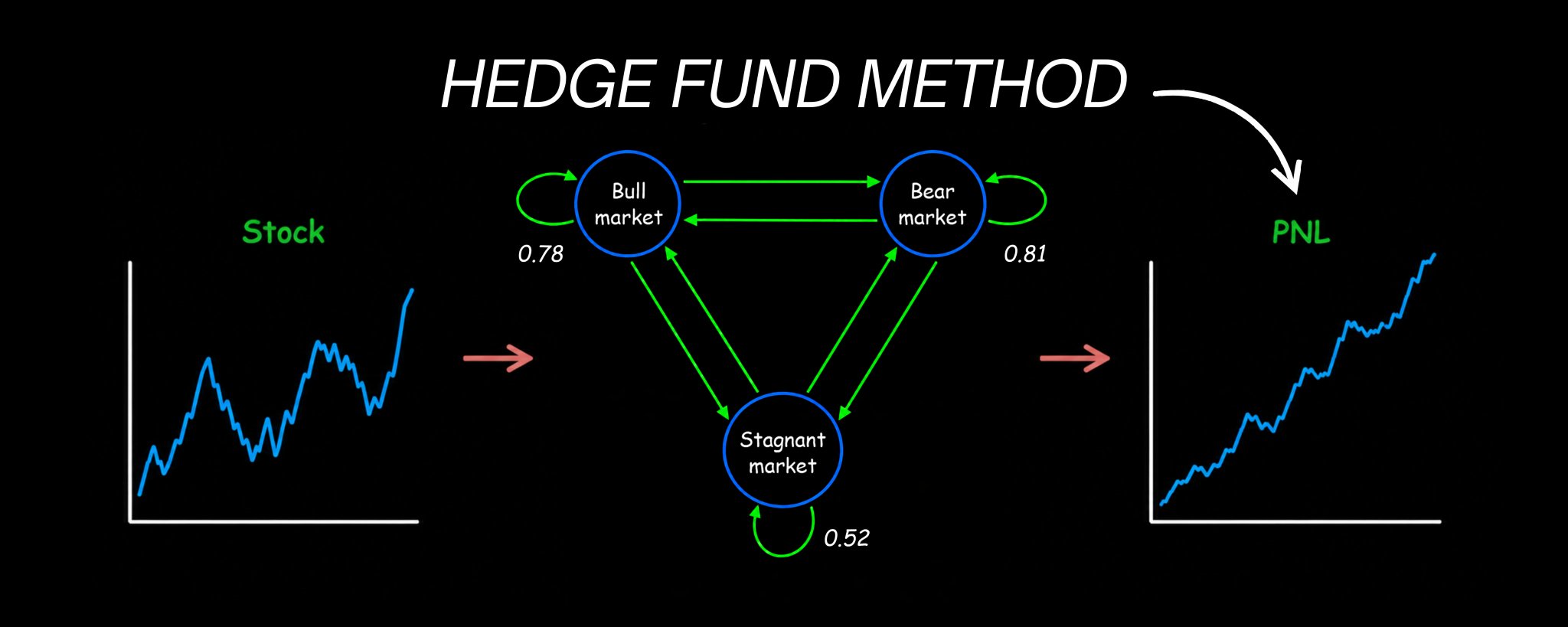
Quants look at the same chart and see something completely different. They see a sequence of states. Bull. Bear. Sideways. Each state carrying its own probability of persisting or transitioning into the next one. Each transition governed by mathematics that has been used to model everything from loan defaults to DNA sequences to Google’s original PageRank algorithm.

The framework is called a Markov Chain. And it is one of the most versatile and underused tools in systematic trading.

While most retail traders are drawing support lines and watching RSI, the quantitative research teams at firms like Citadel and Two Sigma are building regime-switching models that understand not just where the market is, but where it is most likely to go next based on where it has been. The math behind those models starts exactly here.

I have already written the complete neural networks implementation framework for building machine learning trading signals. That article is the next logical companion to this one.

May 6

By the end of this article you will understand exactly what a Markov Chain is and why it maps market behavior better than any single indicator, how to build a complete state transition model from real market data, how to compute the probability of any future market state using nothing more than matrix multiplication, the complete implementation pipeline from raw price data to live trading signals, and the exact mistakes that cause most Markov Chain models to fail in live markets.

Note: This article is deliberately long. Every part builds on the one before it. If you are serious about adding a genuine quantitative edge to your trading, read every single word. If you are looking for a shortcut, this is not for you.

Part 1: Why Independence Fails and Where Markov Chains Begin

Before you can build anything with Markov Chains, you need to understand the fundamental problem they were designed to solve.

Most basic probability models assume independence. Each event is treated as though it has no connection to what came before it. Roll a die. The outcome of roll 100 has nothing to do with roll 99. Each roll is completely independent.

Markets do not work this way.

Imagine you are modeling a portfolio of loans. Each loan at any point in time can be in one of four states: current, 30 to 59 days late, 60 to 89 days late, or 90 plus days late. You want to model how this portfolio evolves over time. So you try the simplest approach. You model each month independently. You draw from each state’s historical distribution.

One month later, your model says that some loans that were current last month are now 90 plus days delinquent.

That is mathematically impossible. A loan cannot jump from current to 90 plus days late in a single 30-day period. The naive independence assumption produced a model that violates reality.

This is exactly the problem Markov Chains solve. Instead of assuming each step is independent of everything that came before it, a Markov Chain introduces local conditional dependence. The next state depends on the current state. Not on everything that happened ten steps ago. Just on where you are right now.

Formally, a sequence of random variables X₀, X₁, X₂, … is a Markov Chain if it satisfies the Markov property:

P(Xₙ₊₁ = s | X₀, X₁, …, Xₙ) = P(Xₙ₊₁ = s | Xₙ)

The probability of the next state depends only on the current state, not on the entire history. This single property is what makes Markov Chains simultaneously tractable and powerful. They capture the essential dependency structure of a process without requiring you to track the entire history.

For financial markets, this translates directly. The probability that the market will be in a bull regime next month depends on whether it is in a bull, bear, or sideways regime this month. Not on what happened two years ago. The current state carries all the relevant information you need to forecast the next state.

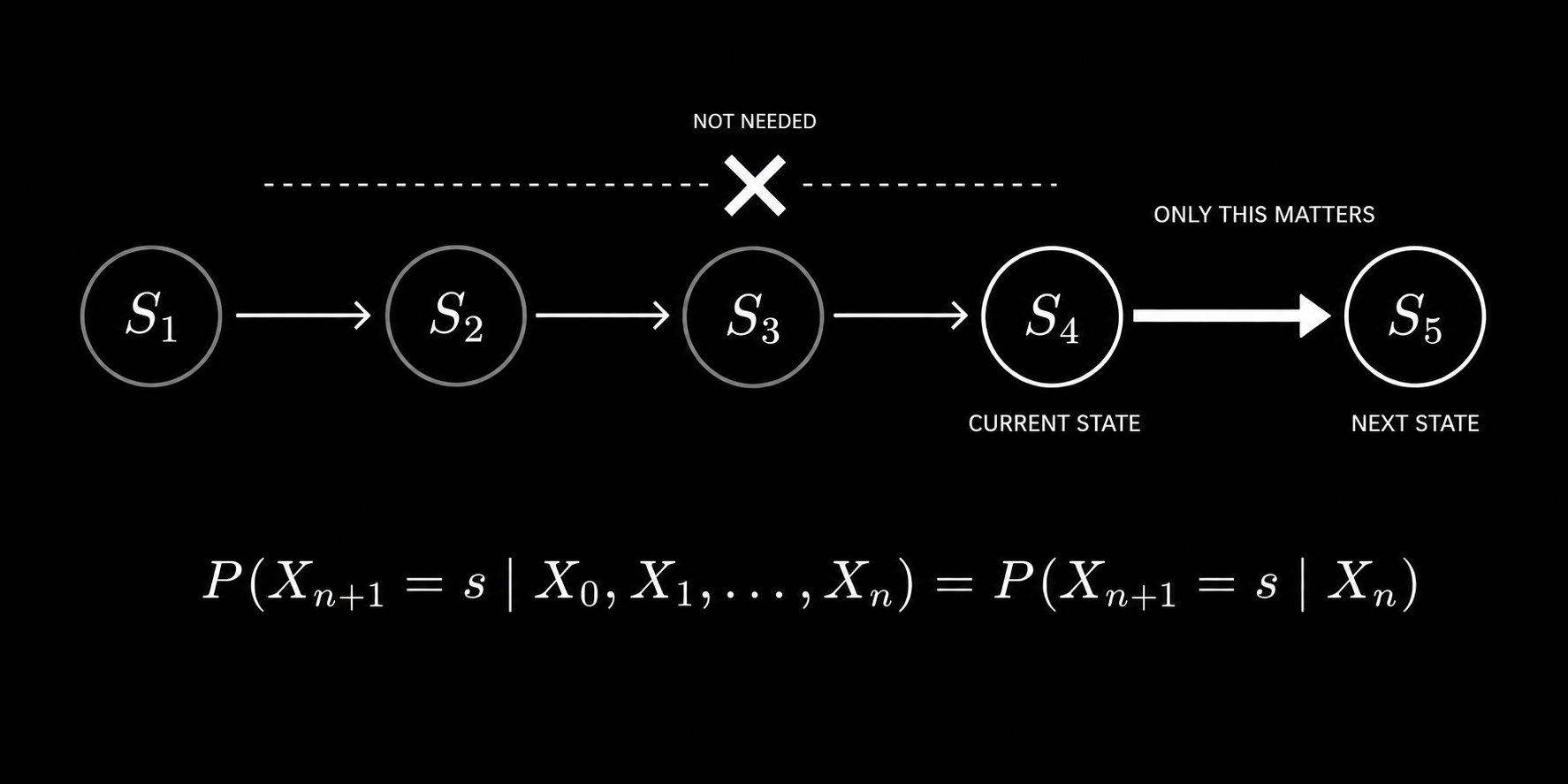
The Markov property states that the probability of the next state depends only on the current state, not on the full history of past states.

This is not a simplification made for convenience. It is a mathematically principled assumption that, when applied correctly, produces models that are dramatically more accurate than naive independence while remaining computationally tractable.

Part 2: Building the State Space and Transition Matrix

The first practical step in building a Markov Chain trading model is defining your states. This is more important than most practitioners realize.

For financial markets, common state definitions include:

Volatility regimes: Low volatility, medium volatility, high volatility defined by rolling realized volatility thresholds. Trend regimes: Bull, bear, sideways defined by the position of price relative to moving averages or by the sign and magnitude of recent returns. Liquidity regimes: High liquidity, low liquidity defined by bid-ask spreads or order book depth. Credit regimes: Risk-on, risk-off defined by credit spreads or cross-asset correlations.

For a concrete starting implementation, a three-state market regime model works well. Define:

State 0 as Bull: the 20-day return is above a positive threshold. State 1 as Bear: the 20-day return is below a negative threshold. State 2 as Sideways: everything in between.

The key requirement is that your states must be mutually exclusive and collectively exhaustive. Every observation must fall into exactly one state at any point in time. No gaps and no overlaps.

Once you have defined your states, you need to estimate the transition probabilities between them. This is the transition matrix. Each entry P(i,j) represents the probability of moving from state i to state j in one time step.

The transition matrix for a three-state model looks like this:

P = | P(0,0) P(0,1) P(0,2) | | P(1,0) P(1,1) P(1,2) | | P(2,0) P(2,1) P(2,2) |

Each row must sum to exactly 1.0 because from any given state, the system must transition to some state in the next step, including staying in the same state.

The maximum likelihood estimator for each transition probability is beautifully simple. Count how many times the system transitioned from state i to state j. Divide by the total number of transitions out of state i:

P̂(i,j) = Count(i → j) / Count(i → any state)

This is exactly how you would intuitively estimate a probability. It is also what the full derivation of the maximum likelihood estimator produces when you maximize the log-likelihood function for Markov Chain data. The intuitive answer and the mathematically rigorous answer are the same.

Here is the complete Python implementation:

import numpy as np
import pandas as pd
import yfinance as yf

def define_market_states(returns, bull_threshold=0.02, bear_threshold=-0.02, window=20):
    rolling_return = returns.rolling(window).sum()
    states = np.where(rolling_return > bull_threshold, 0,
             np.where(rolling_return < bear_threshold, 1, 2))
    return pd.Series(states, index=returns.index)

def estimate_transition_matrix(states, n_states=3):
    transition_counts = np.zeros((n_states, n_states))
    state_values = states.dropna().values
    
    for i in range(len(state_values) - 1):
        current_state = int(state_values[i])
        next_state = int(state_values[i + 1])
        if not np.isnan(current_state) and not np.isnan(next_state):
            transition_counts[current_state][next_state] += 1
    
    transition_matrix = np.zeros((n_states, n_states))
    for i in range(n_states):
        row_sum = transition_counts[i].sum()
        if row_sum > 0:
            transition_matrix[i] = transition_counts[i] / row_sum
    
    return transition_matrix

ticker = yf.Ticker("SPY")
df = ticker.history(period="10y", interval="1d")
returns = df['Close'].pct_change().dropna()

states = define_market_states(returns)
P = estimate_transition_matrix(states)

state_names = ['Bull', 'Bear', 'Sideways']
print("Transition Matrix:")
print(pd.DataFrame(P, index=state_names, columns=state_names).round(3))

The transition matrix you produce from this process is the map of your market. Every entry tells you the probability of moving between two specific regimes. It is the foundation of everything that follows.

Part 3: Computing Multi-Step Transition Probabilities

This is where Markov Chains become genuinely powerful as a trading tool.

You now have the one-step transition matrix P. But what you really want to know as a trader is not just what happens next month. You want to know what the market is likely to look like in three months, six months, twelve months. You want to know the probability of starting in a bull regime today and ending up in a bear regime after twelve transitions.

This is where the Chapman-Kolmogorov equation comes in. It states that the n-step transition probability from state i to state j is the (i,j) entry of the matrix P raised to the nth power:

P^(n)(i,j) = [Pⁿ]ᵢⱼ

That is it. To compute the probability of transitioning from any state to any other state in n steps, you simply multiply the transition matrix by itself n times and read the corresponding entry.

This is an extraordinarily elegant result. All the mathematical complexity of computing paths through a state space over multiple steps reduces to a single matrix power.

def multi_step_transition(P, n_steps):
    return np.linalg.matrix_power(P, n_steps)

def regime_probability_forecast(P, current_state, n_steps, state_names):
    P_n = multi_step_transition(P, n_steps)
    probabilities = P_n[current_state]
    
    print(f"\nFrom {state_names[current_state]} regime:")
    print(f"After {n_steps} steps:")
    for i, (name, prob) in enumerate(zip(state_names, probabilities)):
        print(f"  Probability of {name}: {prob:.4f}")
    
    return probabilities

state_names = ['Bull', 'Bear', 'Sideways']

for steps in [1, 5, 12, 24]:
    regime_probability_forecast(P, current_state=0, n_steps=steps, state_names=state_names)

What this tells you as a trader is specific and actionable. If you are currently in a bull regime, you can now quantify the probability that you will still be in a bull regime in 12 months versus having transitioned to bear or sideways. That probability informs your position sizing, your hedging decisions, and your strategy allocation.

There is another critical output from this framework: the stationary distribution. As n becomes very large, the distribution across states converges to a fixed vector π regardless of the starting state:

π = π × P

The stationary distribution tells you the long-run proportion of time the market spends in each regime. In practice, you solve for π using:

def find_stationary_distribution(P):
    n = P.shape[0]
    A = (P.T - np.eye(n))
    A[-1] = 1
    b = np.zeros(n)
    b[-1] = 1
    
    pi = np.linalg.solve(A, b)
    return pi

pi = find_stationary_distribution(P)
state_names = ['Bull', 'Bear', 'Sideways']
print("\nStationary Distribution:")
for name, prob in zip(state_names, pi):
    print(f"  {name}: {prob:.4f}")

The stationary distribution is your long-run baseline. Any strategy that bets heavily on a regime that the stationary distribution tells you is rare is taking on significant tail risk. Knowing the long-run regime proportions is essential for strategy design.

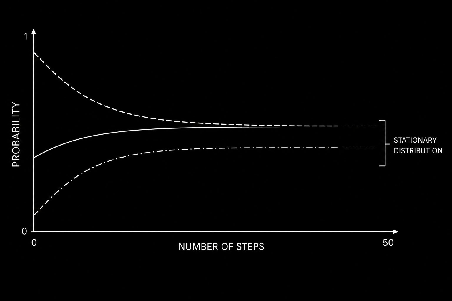
Regardless of starting state, the probability distribution across regimes converges to a fixed stationary distribution as the number of steps increases.

Part 4: From Regime Model to Trading Signal

Having a regime model is not a trading strategy. Converting it into one requires connecting the regime probabilities to specific position decisions.

The core insight is this: the Markov Chain gives you a probability distribution over future states at each point in time. Your trading signal is a function of that distribution.

The simplest approach is direct regime-based allocation. When the model says you are in a bull regime, go long. When bear, go short or flat. When sideways, reduce position size.

A more sophisticated approach uses the full probability vector as input to position sizing. The current state distribution vector π_t represents your probability allocation across regimes at time t. You can construct a position that is proportional to your confidence in each regime:

def compute_trading_signal(current_state, P, strategy_returns_by_regime):
    one_step = P[current_state]
    
    bull_prob = one_step[0]
    bear_prob = one_step[1]
    sideways_prob = one_step[2]
    
    signal = bull_prob - bear_prob
    
    if signal > 0.3:
        position = 1.0
    elif signal < -0.3:
        position = -1.0
    elif abs(signal) < 0.1:
        position = 0.0
    else:
        position = signal / 0.3
    
    return position, one_step

def backtest_markov_strategy(returns, states, P, lookback=252):
    positions = []
    dates = []
    
    state_values = states.dropna()
    
    for i in range(lookback, len(state_values)):
        historical_states = state_values.iloc[i-lookback:i]
        P_estimated = estimate_transition_matrix(historical_states)
        
        current_state = int(state_values.iloc[i])
        position, probs = compute_trading_signal(current_state, P_estimated, None)
        
        positions.append(position)
        dates.append(state_values.index[i])
    
    positions_series = pd.Series(positions, index=dates)
    strategy_returns = positions_series.shift(1) * returns.loc[dates]
    
    sharpe = strategy_returns.mean() / strategy_returns.std() * np.sqrt(252)
    
    cumulative = (1 + strategy_returns).cumprod()
    rolling_max = cumulative.cummax()
    max_drawdown = ((cumulative - rolling_max) / rolling_max).min()
    
    print(f"Annualized Sharpe: {sharpe:.4f}")
    print(f"Maximum Drawdown: {max_drawdown:.4f}")
    print(f"Annual Return: {strategy_returns.mean() * 252:.4f}")
    
    return strategy_returns, positions_series

The walk-forward structure in the backtest above is critical. You re-estimate the transition matrix at each step using only the historical data available at that point. You never use future information to estimate past probabilities. This is the difference between a realistic backtest and one that is guaranteed to disappoint in live trading.

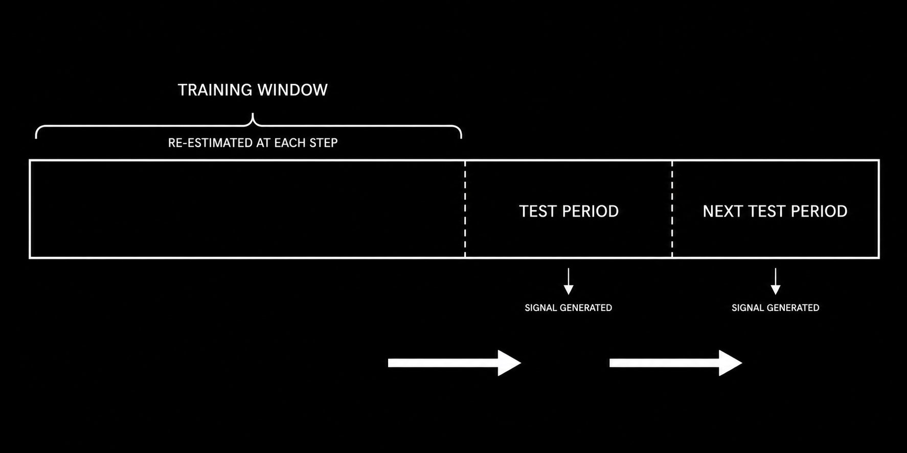
The walk-forward structure ensures the transition matrix is estimated only from data available at each point in time, preventing lookahead bias.

Part 5: The Complete Implementation Pipeline and Critical Limitations

This section assembles everything into a production-ready Markov Chain trading system and addresses the assumptions that will determine whether your model survives contact with live markets.

Complete system implementation:

import numpy as np
import pandas as pd
import yfinance as yf
from sklearn.preprocessing import StandardScaler
import warnings
warnings.filterwarnings('ignore')

class MarkovChainTradingSystem:
    def __init__(self, n_states=3, lookback_window=252, regime_window=20):
        self.n_states = n_states
        self.lookback_window = lookback_window
        self.regime_window = regime_window
        self.transition_matrix = None
        self.state_names = ['Bull', 'Bear', 'Sideways']
    
    def fetch_data(self, ticker, period="10y"):
        data = yf.Ticker(ticker).history(period=period, interval="1d")
        self.returns = data['Close'].pct_change().dropna()
        self.prices = data['Close']
        return self.returns
    
    def label_states(self, returns, bull_thresh=0.02, bear_thresh=-0.02):
        rolling_ret = returns.rolling(self.regime_window).sum()
        states = np.where(rolling_ret > bull_thresh, 0,
                 np.where(rolling_ret < bear_thresh, 1, 2))
        return pd.Series(states, index=returns.index)
    
    def estimate_transition_matrix(self, states):
        counts = np.zeros((self.n_states, self.n_states))
        vals = states.dropna().values.astype(int)
        for i in range(len(vals) - 1):
            if 0 <= vals[i] < self.n_states and 0 <= vals[i+1] < self.n_states:
                counts[vals[i]][vals[i+1]] += 1
        P = np.zeros_like(counts)
        for i in range(self.n_states):
            if counts[i].sum() > 0:
                P[i] = counts[i] / counts[i].sum()
        return P
    
    def stationary_distribution(self, P):
        n = P.shape[0]
        A = (P.T - np.eye(n))
        A[-1] = 1
        b = np.zeros(n)
        b[-1] = 1
        try:
            return np.linalg.solve(A, b)
        except:
            return np.ones(n) / n
    
    def generate_signal(self, P, current_state):
        probs = P[current_state]
        return probs[0] - probs[1]
    
    def run_walkforward_backtest(self):
        states = self.label_states(self.returns)
        signals = []
        
        for i in range(self.lookback_window, len(states)):
            historical = states.iloc[i - self.lookback_window:i]
            P = self.estimate_transition_matrix(historical)
            current = int(states.iloc[i])
            signal = self.generate_signal(P, current)
            signals.append({'date': states.index[i], 'signal': signal,
                           'state': self.state_names[current]})
        
        signals_df = pd.DataFrame(signals).set_index('date')
        position = np.sign(signals_df['signal'])
        position[abs(signals_df['signal']) < 0.1] = 0
        
        strategy_returns = position.shift(1) * self.returns.loc[signals_df.index]
        
        sharpe = strategy_returns.mean() / strategy_returns.std() * np.sqrt(252)
        cumulative = (1 + strategy_returns).cumprod()
        max_dd = ((cumulative - cumulative.cummax()) / cumulative.cummax()).min()
        
        print(f"\nMarkov Chain Trading System Results:")
        print(f"Annualized Sharpe Ratio: {sharpe:.4f}")
        print(f"Maximum Drawdown: {max_dd:.4f}")
        print(f"Annualized Return: {strategy_returns.mean() * 252:.4f}")
        print(f"\nRegime Distribution:")
        print(signals_df['state'].value_counts(normalize=True).round(3))
        
        return strategy_returns, signals_df

system = MarkovChainTradingSystem()
system.fetch_data("SPY")
returns, signals = system.run_walkforward_backtest()

The three assumptions you must understand before deploying:

The first is the Markov property itself. The model assumes that the next state depends only on the current state, not on longer history. In reality, markets sometimes exhibit longer-range dependencies. A trend that has been running for six months may have different transition probabilities than one that just started. You can partially address this by expanding your state space to include duration information, though this increases complexity significantly.

The second is time homogeneity. The model assumes transition probabilities are constant over time. They are not. The probability of a bull regime transitioning to bear was very different in 2008 than in 2021. The standard mitigation is rolling window re-estimation, which you have already seen in the walk-forward backtest above. Shorter windows adapt faster but produce noisier estimates. Longer windows produce more stable estimates but lag regime changes.

The third is sufficient data for reliable estimation. The maximum likelihood estimator converges to true transition probabilities as you observe more transitions. With few observations, particularly for rare transitions, your estimates will be noisy and unreliable. Always check that every cell in your transition matrix has been estimated from at least 20 to 30 observed transitions. If not, consider merging states or extending your data history.

Part 6: Hidden Markov Models - Taking the Framework Further

Every assumption in the model so far has one thing in common. You assumed you could see the regime.

You labeled each day as Bull, Bear, or Sideways using rolling returns. But the regime was never directly observable. You reverse engineered it from price. That is not the same thing. A bear regime that has not yet shown up in prices because institutional positioning is quietly shifting beneath the surface is completely invisible to your state labels. This is the core limitation of observable Markov Chains. Hidden Markov Models fix it.

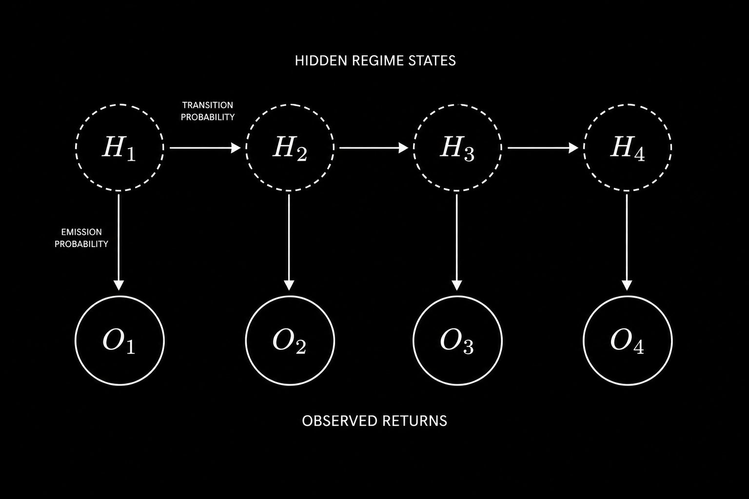
In a Hidden Markov Model, the true market regime is unobservable. Only noisy return observations are available, from which the hidden regime sequence must be inferred.

In an HMM, the true regime is a hidden state you cannot observe. What you can observe is the returns sequence. Each hidden state generates returns from its own distribution. The bull regime produces returns with a positive mean and low variance. The bear regime produces returns with a negative mean and high variance. The model learns both the regime transitions and the return distributions at the same time, from price data alone, without you ever labeling a single day by hand.

There are two algorithms that make this work.

The first is Baum-Welch. This is the algorithm that estimates all model parameters from the observable return sequence. You give it returns. It learns the transition matrix, the return distribution for each regime, and the starting probabilities, all without requiring labeled data. It runs forward through the sequence computing probabilities, then backward to refine them, repeating until convergence.

The second is Viterbi. Once you have a fitted model, Viterbi decodes the most likely sequence of hidden regimes that produced your observed returns. It does not give you soft probabilities. It gives you the single best path through the hidden state space.

from hmmlearn import hmm
import numpy as np
import pandas as pd

def fit_market_hmm(returns, n_states=3, n_iter=1000):
    X = returns.values.reshape(-1, 1)
    
    model = hmm.GaussianHMM(
        n_components=n_states,
        covariance_type="full",
        n_iter=n_iter,
        random_state=42
    )
    model.fit(X)
    
    hidden_states = model.predict(X)
    
    state_means = {s: returns[hidden_states == s].mean() for s in range(n_states)}
    sorted_states = sorted(state_means, key=state_means.get, reverse=True)
    state_map = {old: new for new, old in enumerate(sorted_states)}
    labeled = np.array([state_map[s] for s in hidden_states])
    
    print("Learned Transition Matrix:")
    print(np.round(model.transmat_, 3))
    
    state_names = ['Bull', 'Bear', 'Sideways']
    for i in range(n_states):
        mask = labeled == i
        print(f"{state_names[i]}: mean={returns[mask].mean():.4f}, vol={returns[mask].std():.4f}")
    
    return model, labeled

model, labeled_states = fit_market_hmm(returns)

The signal generation is identical to Part 4. At each step you compute the probability of being in each regime right now. You multiply that vector by the transition matrix to get the one step ahead forecast. Bull probability minus bear probability gives your position.

def hmm_signal(model, returns, lookback=252):
    signals = []
    
    for i in range(lookback, len(returns)):
        window = returns.iloc[i - lookback:i].values.reshape(-1, 1)
        posteriors = model.predict_proba(window)
        current_probs = posteriors[-1]
        next_probs = current_probs @ model.transmat_
        signals.append(next_probs[0] - next_probs[1])
    
    return pd.Series(signals, index=returns.index[lookback:])

Two things to keep in mind before you deploy this. Baum-Welch finds a local maximum, not a global one. Always run it from multiple random starts and keep the model with the highest log likelihood. The default single initialization will frequently produce suboptimal regime assignments. The emission variables you choose matter more than any other design decision. Returns alone carry limited information about the true economic regime. Returns combined with realized volatility, credit spreads, and VIX term structure give the model a much richer signal. The choice of what to feed as observations is where domain knowledge compounds the mathematics.

The observable Markov Chain gave you a regime map. The Hidden Markov Model builds that map in real time from noisy signals, without requiring a single manually labeled data point. That is the direction institutional regime switching models have moved. You now have the complete framework to build one.

The Summary

Markov Chains do not predict the future. What they do is something more useful. They quantify the probability of every possible future state given the current state. They give you a mathematical map of market regimes and the likelihood of transitioning between them.

The framework is fully implementable in a weekend. The transition matrix is estimated from historical data in a handful of lines of Python. The Chapman-Kolmogorov equation gives you n-step forecasts through a single matrix power. The stationary distribution tells you the long-run baseline. And the walk-forward backtest tells you whether your model has genuine predictive power or is fitting noise.

The assumptions are real and they matter. Time homogeneity is violated. The Markov property is an approximation. Estimation error is always present. But as a first pass model and as a building block for more sophisticated Hidden Markov Model extensions, this framework has been deployed in production at real firms and has generated real edge.

You now have the complete implementation. The code is in this article. The mathematics is explained from first principles. The critical limitations are documented so you know exactly where the model can fail and how to mitigate those failures.

Here is the question I want you to sit with.

The Markov Chain model defines regimes based on observable price behavior. But the most important market regimes, the ones that institutional traders actually trade around, are often driven by latent factors like credit conditions, monetary policy stance, and risk appetite that are not directly visible in price data alone. If you were designing a Hidden Markov Model for markets, what observable signals would you use as your emission variables and why?

Drop your answer in the comments.

There is no wrong answer but there are very revealing ones.

Source

Written by @RohOnChain · View original post · Published: 2026-05-06